tolerance <- 0.05Appendix B — Near Equality Tests
This document provides unit tests for the LogoClim NetLogo model. The tests perform near-equality comparisons to validate tolerance expectations during the processing of WorldClim data in NetLogo.
B.1 Problem
LogoClim integrates WorldClim data into NetLogo models through a multi-step conversion process. WorldClim provides raster data in GeoTIFF format, a high-precision binary format for geospatial data, but NetLogo’s GIS extension requires data in Esri ASCII format, a text-based format that stores values with limited decimal precision. This conversion can introduce numerical differences through two main sources:
- Decimal precision loss: Esri ASCII files store values as text with a fixed number of decimal places, rounding continuous values from the original GeoTIFF.
- Spatial interpolation: When NetLogo’s patch grid doesn’t perfectly align with the raster resolution, the GIS extension applies interpolation that may alter cell values.
These discrepancies propagate to summary statistics when comparing the original WorldClim GeoTIFF data with values extracted from LogoClim patches. The unit tests in this document verify that such differences remain within acceptable tolerance levels, ensuring the reliability of downstream simulations and analyses.
B.2 Methods
B.2.1 Source of Data
Data used in this report come from the following sources:
-
WorldClim
- Historical Climate Data series, including 12 monthly data points representing long-term average climate conditions for the period 1970-2000 (Fick & Hijmans, 2017). It provides averages on minimum, mean, and maximum temperature, precipitation, solar radiation, wind speed, vapor pressure, elevation, and on bioclimatic variables.
- Historical Monthly Weather Data series, including 12 monthly data points for each year from 1951 to 2024. Based on downscaled data from CRU-TS-4.09 (Harris et al., 2020), developed by the Climatic Research Unit at the University of East Anglia. It provides monthly averages for minimum temperature, maximum temperature, and total precipitation.
- Future Climate Data series, including 12 monthly data points from downscaled climate projections derived from CMIP6 models (Eyring et al., 2016) for four future periods: 2021-2040, 2041-2060, 2061-2080, and 2081-2100. The projections cover four SSPs (126, 245, 370, and 585), with data available for average minimum temperature, average maximum temperature, total precipitation, and bioclimatic variables.
-
GADM: Database of Global Administrative Areas
- Data on administrative boundaries and regions (Hijmans, n.d.), utilized for plotting country boundaries and cropping raster datasets.
B.2.2 Data Munging
The data munging followed the data science workflow outlined by Wickham et al. (2023), as illustrated in Figure B.1. All processes were made using the Quarto publishing system (Allaire et al., n.d.), the NetLogo environment, the R programming language (R Core Team, n.d.), and several R packages.
For data manipulation and workflow, priority was given to packages from the Tidyverse, rOpenSci and rspatial ecosystems, as well as other packages adhering to the tidy tools manifesto (Wickham, 2023).
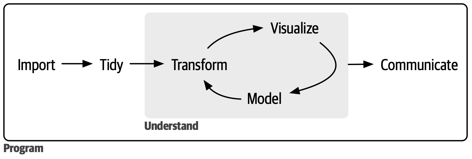
Source: Reproduced from Wickham et al. (2023).
B.2.3 Data Extraction and Transformation
Data extraction was performed using the worldclim_download() function from the orbis R package (Vartanian, 2026c). This function scrapes climate data from the WorldClim website and downloads the relevant GeoTIFF files for the specified variables and time periods.
Following the extraction, the transformation from GeoTIFF to Esri ASCII format is carried out using the worldclim_to_ascii() function from the orbis R package.
B.2.4 NetLogo Integration
Integration with NetLogo (Wilensky, 1999) is facilitated by the logolink R package (Vartanian, 2026b). This package enables the execution of BehaviorSpace experiments directly from R.
Output is extracted in Table and Lists format, containing values, latitude, and longitude for patches, along with global variables that describe the model’s settings.
No Java dependencies are required. NetLogo bundles its own Java Runtime Environment (JRE), ensuring independent operation regardless of the system’s Java installation.
B.2.5 Continuous Integration
The tests use the latest release of NetLogo and are automated using GitHub Actions provided by the LogoActions project (Vartanian, 2026a). Each commit to the code repository triggers test execution, ensuring that changes to the codebase are validated against defined tolerance levels.
B.2.6 Near Equality Tests
The data validation is performed using error tolerance tests with expectations functions from the testthat R package (Wickham, 2011). These tests compare the number of observations (n), minimum, mean, and maximum value of the WorldClim data loaded in LogoClim against the original WorldClim dataset.
Each test begins by selecting a random country to crop the WorldClim data. For each of the three WorldClim series, a random combination of variable, month, year, and other series-specific parameters is drawn using the worldclim_random() function from the orbis R package. No seed is set for the random number generator, so results vary between runs.
Elevation, bioclimatic variables, and the models FIO-ESM-2-0, GFDL-ESM4, and HadGEM3-GC31-LL are excluded due to their data limitations.
B.2.6.1 Minimum Number of Cells
To ensure valid statistical analysis, a minimum number of cells is required. Resolution for each country was determined based on its area, aiming to achieve approximately 1,000 cells. This calculation considers the available resolutions and their approximate cell areas at the Equator:
- 10 minutes (~340 km² per cell)
- 5 minutes (~85 km² per cell)
- 2.5 minutes (~21 km² per cell)
- 30 seconds (~1 km² per cell)
Micronations, like Dominica, were excluded from the analysis due to their small size and limited data availability.
B.2.6.2 Tolerance Level
The all.equal and testthat expect_equal functions were used to perform near-equality tests, both relying on relative tolerance. Comparisons are conducted between the original GeoTIFF file and patch values extracted directly from the LogoClim model.
Relative tolerance is proportional to the value of the quantity being measured. The principle is that larger values can tolerate larger errors.
Given \(x\) and \(y\), relative tolerance can be expressed as:
\[ |x - y| \leq \text{tolerance} \times \max(|x|, |y|) \]
or
\[ \text{tolerance} \geq \frac{|x - y|}{\max(|x|, |y|)} \]
where:
- \(x\) and \(y\) are the values being compared
- \(\text{tolerance}\) is the relative tolerance level
- \(\max(|x|, |y|)\) is the maximum absolute value of \(x\) and \(y\)
For this analysis, the following tolerance level is used:
This means the absolute difference between the numbers can be up to 5% of the larger number’s magnitude. In other words, \(x\) and \(y\) are considered nearly equal if:
\[ \frac{|x - y|}{\max(|x|, |y|)} \leq 0.05 \]
This tolerance may appear high, but it accounts for the maximum cumulative effects of multiple sources of numerical differences, including edge cases encountered during random testing. In practice, observed differences are expected to be substantially smaller than this threshold, reflecting a high degree of agreement between the datasets.
B.2.7 Code Style
The Tidyverse Tidy Tools Manifesto (Wickham, 2023), code style guide (Wickham, n.d.-a) and design principles (Wickham, n.d.-b) were followed to ensure consistency and enhance readability.
B.2.8 Reproducibility
The pipeline is fully reproducible and can be run again at any time. To ensure consistent results, the renv package (Ushey & Wickham, 2025) was used to manage and restore the R environment. See the README file in the code repository to learn how to run it.
B.3 Set the Environment
B.3.1 Load Packages
library(brandr)
library(checkmate)
library(cli)
library(dplyr)
library(fs)
library(geodata)
library(ggplot2)
library(here)
library(ISOcodes)
library(knitr)
library(leaflet)
library(logolink)
library(magrittr)
library(moments)
library(orbis) # github.com/danielvartan/orbis
library(patchwork)
library(purrr)
library(sf)
library(stringr)
library(terra)
library(testthat)
library(tidyr)
library(tidyterra)
B.3.2 Load Custom Functions
The source code for the functions below can be found in the R directory of the code repository.
here("R", "worldclim_raster.R") |> source()
here("R", "logoclim_raster.R") |> source()
here("R", "print_setup.R") |> source()
here("R", "compare_plots.R") |> source()
here("R", "plot_difference.R") |> source()
here("R", "compare_statistics.R") |> source()
here("R", "test_near_equality.R") |> source()
B.3.3 Set Data Directory
The here R package (Müller, 2025) is used to construct file paths relative to the project root directory, ensuring portability across different systems.
A local temporary directory is used to help with debugging and to avoid access privilege issues that can arise when writing outside the project directory. This is particularly relevant for GitHub Actions when using macOS runners.
if (!dir_exists(data_dir)) {
  dir_create(data_dir)
} else {
  dir_ls(data_dir) |> file_delete()
}
B.3.4 Set Initial Variables
Setting the JAVA_TOOL_OPTIONS is optional, but recommended to avoid unnecessary messages from the Java Media Framework.
Sys.setenv(JAVA_TOOL_OPTIONS = "-Dcom.sun.media.jai.disableMediaLib=true")model_path <- here("nlogox", "logoclim.nlogox")B.4 Select Random Country
B.4.1 Select Country
The list of countries is based on the ISO 3166-1 alpha-3 standard and draw using the ISOcodes R package (Hornik & Buchta, 2025).
country <-
  country_names("alpha 3") |>
  str_subset("ATA", negate = TRUE) |>
  sample(1)
country
#> Isle of Man
#> "IMN"B.4.2 Download Country Shape
The rspatial geodata R package (Hijmans et al., 2024) is used to download country shapes from the GADM database (Hijmans, n.d.).
B.4.3 Calculate Shape Area
This while loop filters out micronations. The country’s area is divided by 21 km², the approximate area of a single cell at 2.5-minute resolution at the Equator. This resolution was chosen because it’s the highest available across all three WorldClim datasets (the Historical Monthly Weather Data series tops out at 2.5 minutes). The division ensures the selected country has enough area to yield at least 1,000 cells for analysis.
shape_area
#> [1] 620199.6686
country
#> Central African Republic
#> "CAF"B.4.4 Visualize Country Shape
The rotate() function from the terra package (Hijmans, 2026) is used to adjust shapes that cross the International Date Line (IDL) (e.g., Russian territory).
This adjustment applies only for visualizing countries on leaflet and does not affect the near-equality tests. The Esri ASCII transformation function (worldclim_to_ascii()), used to prepare data for NetLogo, applies the necessary rotation to ensure proper alignment of the raster data with the model’s patch grid.
idl_countries <- c(
  "FJI",
  "KIR",
  "NZL",
  "RUS",
  "USA"
)leaflet() |>
addProviderTiles(providers$Esri.WorldStreetMap) |>
fitBounds(
lng1 = country_shape_leaflet |>
st_bbox() |>
magrittr::extract("xmin") |>
unname(),
lat1 = country_shape_leaflet |>
st_bbox() |>
magrittr::extract("ymin") |>
unname(),
lng2 = country_shape_leaflet |>
st_bbox() |>
magrittr::extract("xmax") |>
unname(),
lat2 = country_shape_leaflet |>
st_bbox() |>
magrittr::extract("ymax") |>
unname()
) |>
addPolygons(
data = country_shape,
fillColor = "transparent",
color = "blue",
weight = 2,
opacity = 1
)B.5 Test Historical Climate Data
This section performs near-equality tests using WorldClim’s Historical Climate Data series.
B.5.1 Select Random WorldClim Dataset
setup <- worldclim_random("hcd")while (setup$variable %in% c("bioc", "elev")) {
setup <- worldclim_random("hcd")
}setup <-
setup |>
inset2(
"resolution",
case_when(
shape_area / 340 >= 1000 ~
c("10 Minutes (~340 km2 at the Equator)" = "10m"),
shape_area / 85 >= 1000 ~
c("5 Minutes (~85 km2 at the Equator)" = "5m"),
shape_area / 21 >= 1000 ~
c("2.5 Minutes (~21 km2 at the Equator)" = "2.5m"),
TRUE ~
c("30 Seconds (~1 km2 at the Equator)" = "30s")
)
)setup
#> $series
#> Historical Climate Data
#> "hcd"
#>
#> $resolution
#> 10 Minutes (~340 km2 at the Equator)
#> "10m"
#>
#> $variable
#> Average Maximum Temperature (°C)
#> "tmax"
#>
#> $year
#> 1970-2000
#> 1978
#>
#> $month
#> December
#> 12B.5.2 Download Dataset
tif_files <- worldclim_download(
  series = setup$series,
  resolution = setup$resolution,
  variable = setup$variable,
  model = setup$model,
  ssp = setup$ssp,
  year = names(setup$year),
  dir = data_dir,
  connection_timeout = 60,
  max_tries = 3,
  retry_on_failure = TRUE,
  backoff = \(attempt) 5^attempt
)
#> ℹ Scraping WorldClim website
#> ✔ Scraping WorldClim website [292ms]
#>
#> ℹ Calculating file sizes
#> ℹ Total download size (compressed): 35.7M.
#> ℹ Calculating file sizes
✔ Calculating file sizes [345ms]
#>
#> ℹ Creating LICENSE and README files
#> ✔ Creating LICENSE and README files [152ms]
#>
#> ℹ Downloading files
#> ℹ Downloading 1 file to '/home/runner/work/logoclim/logoclim/.data-temp/historical-climate-data'
#> ℹ Downloading files
✔ Downloading files [1.7s]
#>
#> ℹ Unzipping files
#> ✔ Unzipping files [13ms]
B.5.3 Transform Data to Esri ASCII Format
tif_file <-
  tif_files |>
  str_subset(
    paste0(
      "(?<=_)",
      setup$variable |> unname(),
      "_",
      str_pad(
        setup$month,
        width = 2,
        pad = "0"
      )
    )
  )
The dx parameter specifies the degree and direction of data rotation. Negative values rotate the data to the left, while positive values rotate it to the right. This adjustment is applied only for countries crossing the International Date Line (IDL).
asc_file <-
  tif_file |>
  worldclim_to_ascii(
    shape = country_shape,
    dx = if_else(country == "USA", 30, -45)
  )
B.5.4 Run Data in LogoClim
setup_file <- create_experiment(
  name = paste0("WorldClim", ": ", names(setup$series)),
  setup = 'setup false',
  go = NULL,
  metrics = c(
    'index',
    'month',
    'year',
    'files',
    'world-width',
    'world-height',
    'cell-size',
    '[first latitude] of patches',
    '[first longitude] of patches',
    '[value] of patches'
  ),
  constants = list(
    "data-series" = names(setup$series),
    "data-resolution" = names(setup$resolution),
    "climate-variable" = names(setup$variable),
    "start-month" = names(setup$month),
    "start-year" = setup$year,
    "data-path" = data_dir
  )
)
results <-
model_path |>
run_experiment(
setup_file = setup_file,
output = c("table", "lists")
)results |> glimpse()
#> List of 3
#> $ metadata:List of 6
#> ..$ timestamp : POSIXct[1:1], format: "2026-02-26 21:07:12"
#> ..$ netlogo_version : chr "7.0.3"
#> ..$ output_version : chr "2.0"
#> ..$ model_file : chr "logoclim.nlogox"
#> ..$ experiment_name : chr "WorldClim: Historical Climate Data"
#> ..$ world_dimensions: Named int [1:4] -135 135 -117 117
#> .. ..- attr(*, "names")= chr [1:4] "min-pxcor" "max-pxcor" "min-pycor" "max-pycor"
#> $ table : tibble [1 × 18] (S3: tbl_df/tbl/data.frame)
#> ..$ run_number : num 1
#> ..$ data_series : chr "Historical Climate Data"
#> ..$ data_resolution : chr "10 Minutes (~340 km2 at the Equator)"
#> ..$ climate_variable : chr "Average Maximum Temperature (°C)"
#> ..$ start_month : chr "December"
#> ..$ start_year : num 1978
#> ..$ data_path : chr "/home/runner/work/logoclim/logoclim/.data-temp"
#> ..$ step : num 1
#> ..$ index : num 0
#> ..$ month : chr "December"
#> ..$ year : chr "1970-2000"
#> ..$ files : chr "[wc2.1_10m_tmax_1970-2000-12.asc]"
#> ..$ world_width : num 79
#> ..$ world_height : num 54
#> ..$ cell_size : num 0.167
#> ..$ first_latitude_of_patches : chr "[5.833333333341 5.500000000007 2.8333333333349997 11.000000000018 5.166666666673 9.000000000014 2.500000000001 "| __truncated__
#> ..$ first_longitude_of_patches: chr "[14.666666666667 14.5 23.833333333352 24.000000000019 17.333333333339 15.833333333336 23.000000000017 27.000000"| __truncated__
#> ..$ value_of_patches : chr "[30.0252494812012 29.8404998779297 false false 30.7775001525879 false false false false 30.2115001678467 31.398"| __truncated__
#> $ lists : tibble [4,266 × 13] (S3: tbl_df/tbl/data.frame)
#> ..$ run_number : num [1:4266] 1 1 1 1 1 1 1 1 1 1 ...
#> ..$ data_series : chr [1:4266] "Historical Climate Data" "Historical Climate Data" "Historical Climate Data" "Historical Climate Data" ...
#> ..$ data_resolution : chr [1:4266] "10 Minutes (~340 km2 at the Equator)" "10 Minutes (~340 km2 at the Equator)" "10 Minutes (~340 km2 at the Equator)" "10 Minutes (~340 km2 at the Equator)" ...
#> ..$ climate_variable : chr [1:4266] "Average Maximum Temperature (°C)" "Average Maximum Temperature (°C)" "Average Maximum Temperature (°C)" "Average Maximum Temperature (°C)" ...
#> ..$ start_month : chr [1:4266] "December" "December" "December" "December" ...
#> ..$ start_year : num [1:4266] 1978 1978 1978 1978 1978 ...
#> ..$ data_path : chr [1:4266] "/home/runner/work/logoclim/logoclim/.data-temp" "/home/runner/work/logoclim/logoclim/.data-temp" "/home/runner/work/logoclim/logoclim/.data-temp" "/home/runner/work/logoclim/logoclim/.data-temp" ...
#> ..$ step : num [1:4266] 1 1 1 1 1 1 1 1 1 1 ...
#> ..$ index : num [1:4266] 0 1 2 3 4 5 6 7 8 9 ...
#> ..$ files : chr [1:4266] "wc2.1_10m_tmax_1970-2000-12.asc" NA NA NA ...
#> ..$ first_latitude_of_patches : num [1:4266] 5.83 5.5 2.83 11 5.17 ...
#> ..$ first_longitude_of_patches: num [1:4266] 14.7 14.5 23.8 24 17.3 ...
#> ..$ value_of_patches : chr [1:4266] "30.0252494812012" "29.8404998779297" "false" "false" ...B.5.5 Compare Plots
To enable side-by-side comparison in the plots, the LogoClim patch data is resampled to match the WorldClim GeoTIFF grid extent and resolution. This resampling is performed solely for visualization purposes and may introduce minor visual differences between the maps. The statistical comparisons presented in the tables are based on the original data values.
compare_plots(
  tif_file = tif_file,
  country_shape = country_shape,
  results = results,
  setup = setup,
  dx = if_else(country == "USA", 30, -45),
  viridis = FALSE
)
#> ℹ run_numberdata_seriesdata_resolutionclimate_variablestart_monthstart_yeardata_pathstepindexfilesfirst_latitude_of_patchesfirst_longitude_of_patchesvalue_of_patches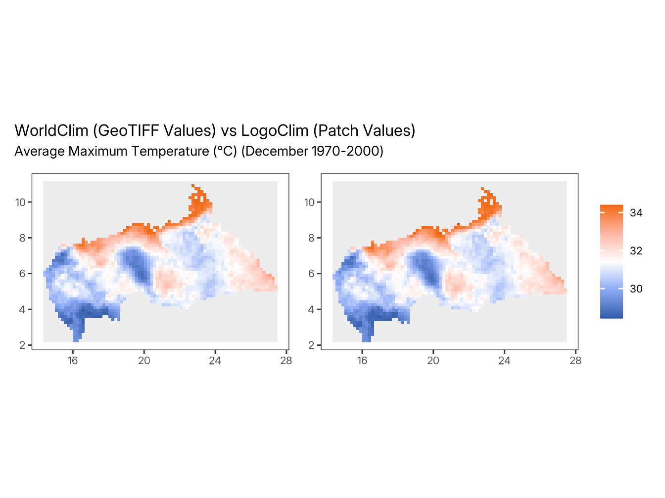
plot_difference(
  tif_file = tif_file,
  country_shape = country_shape,
  results = results,
  setup = setup,
  dx = if_else(country == "USA", 30, -45),
  viridis = FALSE
)
#> ℹ run_numberdata_seriesdata_resolutionclimate_variablestart_monthstart_yeardata_pathstepindexfilesfirst_latitude_of_patchesfirst_longitude_of_patchesvalue_of_patches
B.5.6 Compare Statistics
statistics <- compare_statistics(
  tif_file = tif_file,
  country_shape = country_shape,
  results = results,
  dx = if_else(country == "USA", 30, -45),
  tolerance = tolerance
)statisticsB.5.7 Test Near-Equality
statistics |>
  test_near_equality(
    check = c("n", "min", "mean", "max"),
    tolerance = tolerance
  )
#> ℹ n
#> ✔ n [267ms]
#>
#> ℹ min
#> ✔ min [41ms]
#>
#> ℹ mean
#> ✔ mean [35ms]
#>
#> ℹ max
#> ✔ max [34ms]
#>
B.6 Test Historical Monthly Weather Data
This section performs near-equality tests using WorldClim’s Historical Monthly Weather Data series.
B.6.1 Select Random WorldClim Dataset
setup <- worldclim_random("hmwd")WorldClim’s Historical Monthly Weather Data series does not include the 30 seconds (~1 km² at the Equator) resolution.
setup
#> $series
#> Historical Monthly Weather Data
#>                          "hmwd"
#>
#> $resolution
#> 10 Minutes (~340 km2 at the Equator)
#>                                "10m"
#>
#> $variable
#> Total Precipitation (mm)
#>                   "prec"
#>
#> $year
#> 2020-2024
#>      2023
#>
#> $month
#> July
#>    7
B.6.2 Download Dataset
tif_files <- worldclim_download(
  series = setup$series,
  resolution = setup$resolution,
  variable = setup$variable,
  model = setup$model,
  ssp = setup$ssp,
  year = names(setup$year),
  dir = data_dir,
  connection_timeout = 60,
  max_tries = 3,
  retry_on_failure = TRUE,
  backoff = \(attempt) 5^attempt
)
#> ℹ Scraping WorldClim website
#> ✔ Scraping WorldClim website [49ms]
#>
#> ℹ Calculating file sizes
#> ℹ Total download size (compressed): 104M.
#> ℹ Calculating file sizes
✔ Calculating file sizes [282ms]
#>
#> ℹ Creating LICENSE and README files
#> ✔ Creating LICENSE and README files [17ms]
#>
#> ℹ Downloading files
#> ℹ Downloading 1 file to '/home/runner/work/logoclim/logoclim/.data-temp/historical-monthly-weather-data'
#> ℹ Downloading files
✔ Downloading files [4.4s]
#>
#> ℹ Unzipping files
#> ✔ Unzipping files [13ms]
B.6.3 Transform Data to Esri ASCII Format
tif_file <-
  tif_files |>
  str_subset(
    paste0(
      setup$year,
      "-",
      str_pad(setup$month, width = 2, pad = "0")
    )
  )
The dx parameter specifies the degree and direction of data rotation. Negative values rotate the data to the left, while positive values rotate it to the right. This adjustment is applied only for countries crossing the International Date Line (IDL).
asc_file <-
  tif_file |>
  worldclim_to_ascii(
    shape = country_shape,
    dx = if_else(country == "USA", 30, -45)
  )
B.6.4 Run Data in LogoClim
setup_file <- create_experiment(
  name = paste0("WorldClim", ": ", names(setup$series)),
  setup = 'setup false',
  go = NULL,
  metrics = c(
    'index',
    'month',
    'year',
    'files',
    'world-width',
    'world-height',
    'cell-size',
    '[first latitude] of patches',
    '[first longitude] of patches',
    '[value] of patches'
  ),
  constants = list(
    "data-series" = names(setup$series),
    "data-resolution" = names(setup$resolution),
    "climate-variable" = names(setup$variable),
    "start-month" = names(setup$month),
    "start-year" = setup$year,
    "data-path" = data_dir
  )
)
results <-
model_path |>
run_experiment(
setup_file = setup_file,
output = c("table", "lists")
)results |> glimpse()
#> List of 3
#> $ metadata:List of 6
#> ..$ timestamp : POSIXct[1:1], format: "2026-02-26 21:07:33"
#> ..$ netlogo_version : chr "7.0.3"
#> ..$ output_version : chr "2.0"
#> ..$ model_file : chr "logoclim.nlogox"
#> ..$ experiment_name : chr "WorldClim: Historical Monthly Weather Data"
#> ..$ world_dimensions: Named int [1:4] -135 135 -117 117
#> .. ..- attr(*, "names")= chr [1:4] "min-pxcor" "max-pxcor" "min-pycor" "max-pycor"
#> $ table : tibble [1 × 18] (S3: tbl_df/tbl/data.frame)
#> ..$ run_number : num 1
#> ..$ data_series : chr "Historical Monthly Weather Data"
#> ..$ data_resolution : chr "10 Minutes (~340 km2 at the Equator)"
#> ..$ climate_variable : chr "Total Precipitation (mm)"
#> ..$ start_month : chr "July"
#> ..$ start_year : num 2023
#> ..$ data_path : chr "/home/runner/work/logoclim/logoclim/.data-temp"
#> ..$ step : num 1
#> ..$ index : num 0
#> ..$ month : chr "July"
#> ..$ year : num 2023
#> ..$ files : chr "[wc2.1_cruts4.09_10m_prec_2023-07.asc]"
#> ..$ world_width : num 79
#> ..$ world_height : num 54
#> ..$ cell_size : num 0.167
#> ..$ first_latitude_of_patches : chr "[4.5000000000050004 8.166666666679 4.833333333339 3.333333333336 2.333333333334 10.166666666683 4.166666666671 "| __truncated__
#> ..$ first_longitude_of_patches: chr "[27.166666666692002 26.500000000024002 26.333333333357 21.666666666681 22.83333333335 21.333333333347 24.000000"| __truncated__
#> ..$ value_of_patches : chr "[false false false false false 197.024993896484 false false false 184.274993896484 219.231246948242 222.65625 f"| __truncated__
#> $ lists : tibble [4,266 × 13] (S3: tbl_df/tbl/data.frame)
#> ..$ run_number : num [1:4266] 1 1 1 1 1 1 1 1 1 1 ...
#> ..$ data_series : chr [1:4266] "Historical Monthly Weather Data" "Historical Monthly Weather Data" "Historical Monthly Weather Data" "Historical Monthly Weather Data" ...
#> ..$ data_resolution : chr [1:4266] "10 Minutes (~340 km2 at the Equator)" "10 Minutes (~340 km2 at the Equator)" "10 Minutes (~340 km2 at the Equator)" "10 Minutes (~340 km2 at the Equator)" ...
#> ..$ climate_variable : chr [1:4266] "Total Precipitation (mm)" "Total Precipitation (mm)" "Total Precipitation (mm)" "Total Precipitation (mm)" ...
#> ..$ start_month : chr [1:4266] "July" "July" "July" "July" ...
#> ..$ start_year : num [1:4266] 2023 2023 2023 2023 2023 ...
#> ..$ data_path : chr [1:4266] "/home/runner/work/logoclim/logoclim/.data-temp" "/home/runner/work/logoclim/logoclim/.data-temp" "/home/runner/work/logoclim/logoclim/.data-temp" "/home/runner/work/logoclim/logoclim/.data-temp" ...
#> ..$ step : num [1:4266] 1 1 1 1 1 1 1 1 1 1 ...
#> ..$ index : num [1:4266] 0 1 2 3 4 5 6 7 8 9 ...
#> ..$ files : chr [1:4266] "wc2.1_cruts4.09_10m_prec_2023-07.asc" NA NA NA ...
#> ..$ first_latitude_of_patches : num [1:4266] 4.5 8.17 4.83 3.33 2.33 ...
#> ..$ first_longitude_of_patches: num [1:4266] 27.2 26.5 26.3 21.7 22.8 ...
#> ..$ value_of_patches : chr [1:4266] "false" "false" "false" "false" ...B.6.5 Compare Plots
To enable side-by-side comparison in the plots, the LogoClim patch data is resampled to match the WorldClim GeoTIFF grid extent and resolution. This resampling is performed solely for visualization purposes and may introduce minor visual differences between the maps. The statistical comparisons presented in the tables are based on the original data values.
compare_plots(
  tif_file = tif_file,
  country_shape = country_shape,
  results = results,
  setup = setup,
  dx = if_else(country == "USA", 30, -45),
  viridis = FALSE
)
#> ℹ run_numberdata_seriesdata_resolutionclimate_variablestart_monthstart_yeardata_pathstepindexfilesfirst_latitude_of_patchesfirst_longitude_of_patchesvalue_of_patches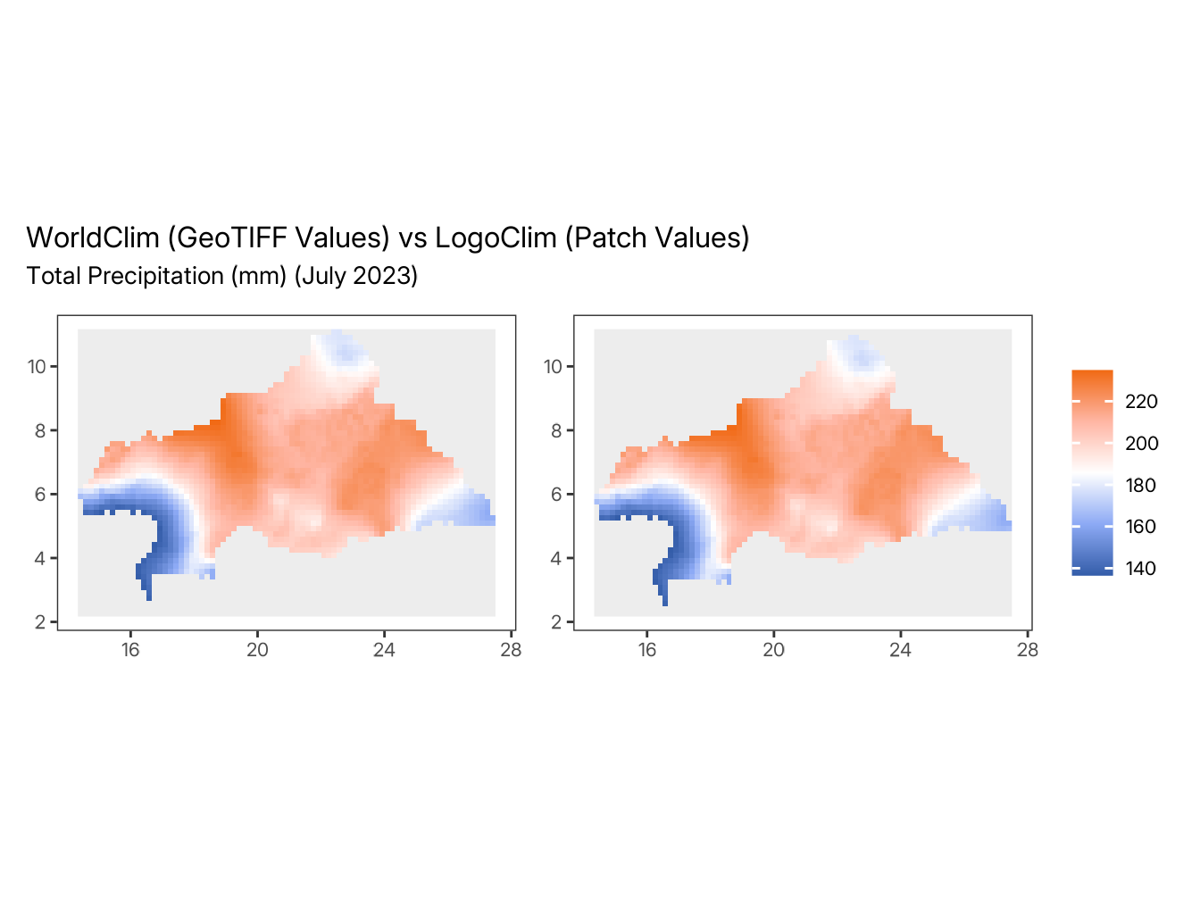
plot_difference(
  tif_file = tif_file,
  country_shape = country_shape,
  results = results,
  setup = setup,
  dx = if_else(country == "USA", 30, -45),
  viridis = FALSE
)
#> ℹ run_numberdata_seriesdata_resolutionclimate_variablestart_monthstart_yeardata_pathstepindexfilesfirst_latitude_of_patchesfirst_longitude_of_patchesvalue_of_patches
B.6.6 Compare Statistics
statistics <- compare_statistics(
  tif_file = tif_file,
  country_shape = country_shape,
  results = results,
  dx = if_else(country == "USA", 30, -45),
  tolerance = tolerance
)statisticsB.6.7 Test Near-Equality
statistics |>
  test_near_equality(
    check = c("n", "min", "mean", "max"),
    tolerance = tolerance
  )
#> ℹ n
#> ✔ n [30ms]
#>
#> ℹ min
#> ✔ min [34ms]
#>
#> ℹ mean
#> ✔ mean [35ms]
#>
#> ℹ max
#> ✔ max [37ms]
#>
B.7 Test Future Climate Data
This section performs near-equality tests using WorldClim’s Future Climate Data series.
B.7.1 Select Random WorldClim Dataset
setup <- worldclim_random("fcd")while (
setup$model %in%
c("FIO-ESM-2-0", "GFDL-ESM4", "HadGEM3-GC31-LL") ||
setup$variable %in% c("bioc")
) {
setup <- worldclim_random("fcd")
}setup <-
setup |>
inset2(
"resolution",
case_when(
shape_area / 340 >= 1000 ~
c("10 Minutes (~340 km2 at the Equator)" = "10m"),
shape_area / 85 >= 1000 ~
c("5 Minutes (~85 km2 at the Equator)" = "5m"),
shape_area / 21 >= 1000 ~
c("2.5 Minutes (~21 km2 at the Equator)" = "2.5m"),
TRUE ~
c("30 Seconds (~1 km2 at the Equator)" = "30s")
)
)setup
#> $series
#> Future Climate Data
#> "fcd"
#>
#> $resolution
#> 10 Minutes (~340 km2 at the Equator)
#> "10m"
#>
#> $variable
#> Average Minimum Temperature (°C)
#> "tmin"
#>
#> $model
#> UK Earth System Model, UK
#> "UKESM1-0-LL"
#>
#> $ssp
#> SSP-126
#> "ssp126"
#>
#> $year
#> 2081-2100
#> 2090
#>
#> $month
#> August
#> 8B.7.2 Download Dataset
tif_file <- worldclim_download(
  series = setup$series,
  resolution = setup$resolution,
  variable = setup$variable,
  model = setup$model,
  ssp = setup$ssp,
  year = names(setup$year),
  dir = data_dir,
  connection_timeout = 60,
  max_tries = 3,
  retry_on_failure = TRUE,
  backoff = \(attempt) 5^attempt
)
#> ℹ Scraping WorldClim website
#> ✔ Scraping WorldClim website [64ms]
#>
#> ℹ Calculating file sizes
#> ℹ Total download size (compressed): 17.1M.
#> ℹ Calculating file sizes
✔ Calculating file sizes [287ms]
#>
#> ℹ Creating LICENSE and README files
#> ✔ Creating LICENSE and README files [19ms]
#>
#> ℹ Downloading files
#> ℹ Downloading 1 file to '/home/runner/work/logoclim/logoclim/.data-temp/future-climate-data'
#> ℹ Downloading files
✔ Downloading files [1.3s]
#>
#> ℹ Unzipping files
#> ✔ Unzipping files [14ms]
B.7.3 Transform Data to Esri ASCII Format
The dx parameter specifies the degree and direction of data rotation. Negative values rotate the data to the left, while positive values rotate it to the right. This adjustment is applied only for countries crossing the International Date Line (IDL).
asc_file <-
  tif_file |>
  worldclim_to_ascii(
    shape = country_shape,
    dx = if_else(country == "USA", 30, -45)
  )
B.7.4 Run Data in LogoClim
setup_file <- create_experiment(
  name = paste0("WorldClim", ": ", names(setup$series)),
  setup = 'setup false',
  go = NULL,
  metrics = c(
    'index',
    'month',
    'year',
    'files',
    'world-width',
    'world-height',
    'cell-size',
    '[first latitude] of patches',
    '[first longitude] of patches',
    '[value] of patches'
  ),
  constants = list(
    "data-series" = names(setup$series),
    "data-resolution" = names(setup$resolution),
    "climate-variable" = names(setup$variable),
    "global-climate-model" = setup$model,
    "shared-socioeconomic-pathway" = names(setup$ssp),
    "start-month" = names(setup$month),
    "start-year" = setup$year,
    "data-path" = data_dir
  )
)
results <-
model_path |>
run_experiment(
setup_file = setup_file,
output = c("table", "lists")
)results |> glimpse()
#> List of 3
#> $ metadata:List of 6
#> ..$ timestamp : POSIXct[1:1], format: "2026-02-26 21:07:49"
#> ..$ netlogo_version : chr "7.0.3"
#> ..$ output_version : chr "2.0"
#> ..$ model_file : chr "logoclim.nlogox"
#> ..$ experiment_name : chr "WorldClim: Future Climate Data"
#> ..$ world_dimensions: Named int [1:4] -135 135 -117 117
#> .. ..- attr(*, "names")= chr [1:4] "min-pxcor" "max-pxcor" "min-pycor" "max-pycor"
#> $ table : tibble [1 × 20] (S3: tbl_df/tbl/data.frame)
#> ..$ run_number : num 1
#> ..$ data_series : chr "Future Climate Data"
#> ..$ data_resolution : chr "10 Minutes (~340 km2 at the Equator)"
#> ..$ climate_variable : chr "Average Minimum Temperature (°C)"
#> ..$ global_climate_model : chr "UKESM1-0-LL"
#> ..$ shared_socioeconomic_pathway: chr "SSP-126"
#> ..$ start_month : chr "August"
#> ..$ start_year : num 2090
#> ..$ data_path : chr "/home/runner/work/logoclim/logoclim/.data-temp"
#> ..$ step : num 1
#> ..$ index : num 0
#> ..$ month : chr "August"
#> ..$ year : chr "2081-2100"
#> ..$ files : chr "[wc2.1_10m_tmin_UKESM1-0-LL_ssp126_2081-2100-08.asc wc2.1_10m_tmin_UKESM1-0-LL_ssp126_2081-2100-09.asc wc2.1_10"| __truncated__
#> ..$ world_width : num 79
#> ..$ world_height : num 54
#> ..$ cell_size : num 0.167
#> ..$ first_latitude_of_patches : chr "[8.333333333346 8.66666666668 9.000000000014 3.833333333337 7.833333333345 9.666666666682 8.500000000013 4.8333"| __truncated__
#> ..$ first_longitude_of_patches : chr "[25.333333333355 19.000000000009 15.500000000002 23.333333333351 14.5 18.000000000007 27.166666666692002 20.500"| __truncated__
#> ..$ value_of_patches : chr "[false 23.2999992370605 false false false false false 22.3999996185303 23 false 23.2000007629395 23.29999923706"| __truncated__
#> $ lists : tibble [4,266 × 15] (S3: tbl_df/tbl/data.frame)
#> ..$ run_number : num [1:4266] 1 1 1 1 1 1 1 1 1 1 ...
#> ..$ data_series : chr [1:4266] "Future Climate Data" "Future Climate Data" "Future Climate Data" "Future Climate Data" ...
#> ..$ data_resolution : chr [1:4266] "10 Minutes (~340 km2 at the Equator)" "10 Minutes (~340 km2 at the Equator)" "10 Minutes (~340 km2 at the Equator)" "10 Minutes (~340 km2 at the Equator)" ...
#> ..$ climate_variable : chr [1:4266] "Average Minimum Temperature (°C)" "Average Minimum Temperature (°C)" "Average Minimum Temperature (°C)" "Average Minimum Temperature (°C)" ...
#> ..$ global_climate_model : chr [1:4266] "UKESM1-0-LL" "UKESM1-0-LL" "UKESM1-0-LL" "UKESM1-0-LL" ...
#> ..$ shared_socioeconomic_pathway: chr [1:4266] "SSP-126" "SSP-126" "SSP-126" "SSP-126" ...
#> ..$ start_month : chr [1:4266] "August" "August" "August" "August" ...
#> ..$ start_year : num [1:4266] 2090 2090 2090 2090 2090 2090 2090 2090 2090 2090 ...
#> ..$ data_path : chr [1:4266] "/home/runner/work/logoclim/logoclim/.data-temp" "/home/runner/work/logoclim/logoclim/.data-temp" "/home/runner/work/logoclim/logoclim/.data-temp" "/home/runner/work/logoclim/logoclim/.data-temp" ...
#> ..$ step : num [1:4266] 1 1 1 1 1 1 1 1 1 1 ...
#> ..$ index : num [1:4266] 0 1 2 3 4 5 6 7 8 9 ...
#> ..$ files : chr [1:4266] "wc2.1_10m_tmin_UKESM1-0-LL_ssp126_2081-2100-08.asc" "wc2.1_10m_tmin_UKESM1-0-LL_ssp126_2081-2100-09.asc" "wc2.1_10m_tmin_UKESM1-0-LL_ssp126_2081-2100-10.asc" "wc2.1_10m_tmin_UKESM1-0-LL_ssp126_2081-2100-11.asc" ...
#> ..$ first_latitude_of_patches : num [1:4266] 8.33 8.67 9 3.83 7.83 ...
#> ..$ first_longitude_of_patches : num [1:4266] 25.3 19 15.5 23.3 14.5 ...
#> ..$ value_of_patches : chr [1:4266] "false" "23.2999992370605" "false" "false" ...B.7.5 Compare Plots
To enable side-by-side comparison in the plots, the LogoClim patch data is resampled to match the WorldClim GeoTIFF grid extent and resolution. This resampling is performed solely for visualization purposes and may introduce minor visual differences between the maps. The statistical comparisons presented in the tables are based on the original data values.
compare_plots(
  tif_file = tif_file,
  country_shape = country_shape,
  results = results,
  setup = setup,
  dx = if_else(country == "USA", 30, -45),
  layer_pattern = setup$month |>
    str_pad(, width = 2, pad = "0") |>
    paste0("$"),
  viridis = FALSE
)
#> ℹ run_numberdata_seriesdata_resolutionclimate_variableglobal_climate_modelshared_socioeconomic_pathwaystart_monthstart_yeardata_pathstepindexfilesfirst_latitude_of_patchesfirst_longitude_of_patchesvalue_of_patches
plot_difference(
  tif_file = tif_file,
  country_shape = country_shape,
  results = results,
  setup = setup,
  dx = if_else(country == "USA", 30, -45),
  layer_pattern = setup$month |>
    str_pad(, width = 2, pad = "0") |>
    paste0("$"),
  viridis = FALSE
)
#> ℹ run_numberdata_seriesdata_resolutionclimate_variableglobal_climate_modelshared_socioeconomic_pathwaystart_monthstart_yeardata_pathstepindexfilesfirst_latitude_of_patchesfirst_longitude_of_patchesvalue_of_patches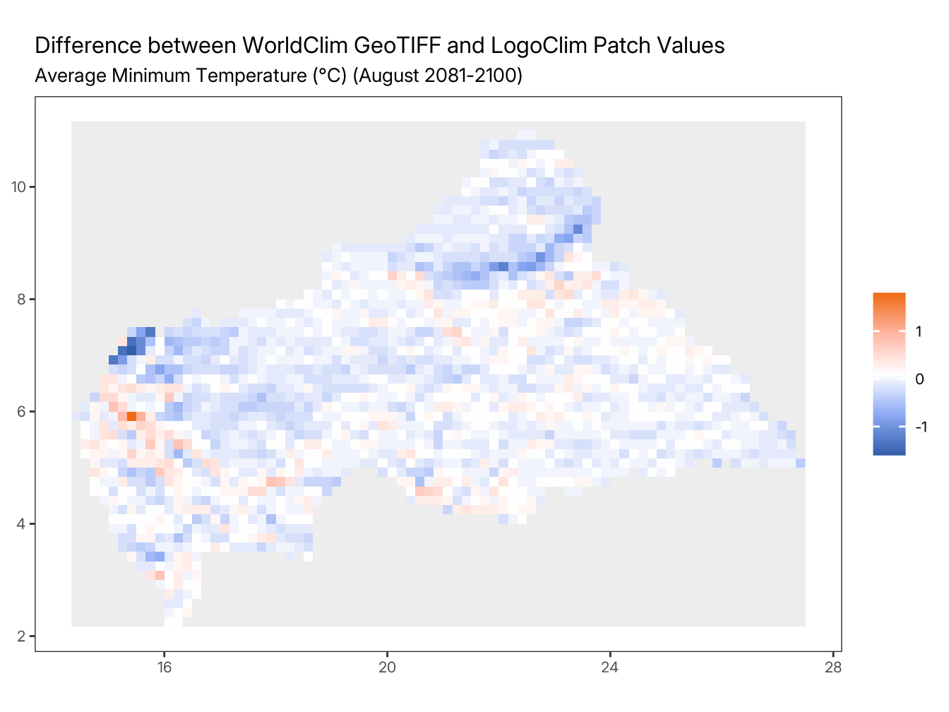
B.7.6 Compare Statistics
statisticsB.7.7 Test Near-Equality
statistics |>
  test_near_equality(
    check = c("n", "min", "mean", "max"),
    tolerance = tolerance
  )
#> ℹ n
#> ✔ n [27ms]
#>
#> ℹ min
#> ✔ min [34ms]
#>
#> ℹ mean
#> ✔ mean [34ms]
#>
#> ℹ max
#> ✔ max [36ms]
#>