2 How to Use It
To get started using LogoClim, you must have NetLogo version 7 or later installed. The NetLogo website provides easy installers for Windows, macOS, and Linux, along with detailed instructions for installation.
The model also depends on four NetLogo extensions: GIS, Pathdir, String, and Time. No manual installation is required since they are automatically installed the first time the model runs.
With NetLogo ready, follow these 5 steps to get LogoClim up and running.
2.1 A. Downloading the Model
You can download the latest release of the model from the CoMSES Network. This is the recommended option for most users, as it provides a stable version of the model that has been tested and documented.
For the development version, you can clone or download the model GitHub code repository directly.
2.2 B. Opening the Model
After downloading and uncompressing the model files, open the logoclim.nlogox file in NetLogo. You can find this file in the code directory when using the CoMSES Network release.
2.3 C. Preparing the Data
The CoMSES Network release includes an example dataset that is ready to use with LogoClim. You can use it as a starting point. But, ideally you should prepare your own data to suit your research needs. The next sections of this manual will guide you through the process of downloading and preparing WorldClim data for use with LogoClim.
We also provide other example datasets for testing and demonstration. These files are available in the model’s OSF repository and are ready to use with LogoClim. Please note that these datasets are for demonstration purposes only and are not be suitable for research applications. Always verify the suitability of the data for your specific research questions and objectives.
2.4 D. Running the Model
With files at hand, use the Select Data Directory button in the model interface to specify their location. This will set the data-path global variable to the correct path, allowing the model to access the data. After that, you can configure the other parameters as needed and start the simulation.
The sections below go through the model interface, explaining the function of each control and how to use it. Once everything is set, click Setup and then Go buttons to start the simulation.
Note that the example dataset included in the CoMSES Network release is intentionally small to keep downloads fast and easy. The model’s default configuration already points to this dataset, so you can simply click Setup and then Go to run the model with it.
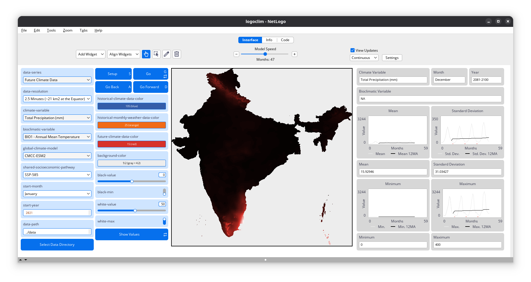
2.4.1 Interface Controls
2.4.1.1 Choosers, Input Boxes, Sliders, And Switches
-
data-series(string): Chooser for selecting a data series (e.g.,"Future Climate Data"). -
data-resolution(string): Chooser for selecting the spatial resolution of the data, expressed in minutes of a degree of latitude/longitude (e.g.,"5 Minutes (~85 km2 at the Equator)"). -
climate-variable(string): Chooser for selecting the climate variable (e.g.,"Average Temperature (°C)"). -
bioclimatic-variable(string): Chooser for selecting a bioclimatic variable (e.g.,"BIO18 - Precipitation of Warmest Quarter"). Only useful whenclimate-variableis set tobioclimatic-variables. -
global-climate-model(string): Chooser for selecting a global climate model (e.g.,"ACCESS-CM2"). Only useful whenFuture Climate Datais selected. -
shared-socioeconomic-pathway(string): Chooser for selecting a Shared Socioeconomic Pathway (SSP) scenario (e.g.,"SSP-370"). Only useful whenFuture Climate Datais selected. -
start-month(string): Chooser for selecting the simulation’s starting month (e.g.,"April"). -
start-year(number): Input box for setting the simulation’s start year inYYYYformat (e.g.1970). -
data-path(string): Input box for setting the path to the data folder. Use theSelect Data Directorybutton to navigate via a dialog window. -
historical-climate-color(number): Input box for setting the color used to represent the Historical Climate Data series. -
historical-monthly-weather-color(number): Input box for setting the color used to represent the Historical Monthly Weather Data series. -
future-climate-color(number): Input box for setting the color used to represent the Future Climate Data series. -
color-bar-bins(number): Slider for setting the number of bins in the Color Bar plot. -
black-value(number): Slider for setting the lower threshold on the world map. -
black-min(boolean): Switch for setting the black color threshold to the minimum value of the current dataset. If it is set toOn,black-valuewill be ignored. -
white-value(number): Slider for setting the upper threshold on the world map. -
white-max(boolean): Switch for setting the white color threshold to the maximum value of the current dataset. If it is set toOn,white-valuewill be ignored.
2.4.2 Monitors And Plots
-
Climate Variable: Displays the climate variable being used. Ifclimate-variableis set to Bioclimatic Variables, it instead shows the variable selected in thebioclimatic-variablechooser. -
Month,Year: Displays the current month and year being simulated. -
Color Bar: A plot showing the color scale used on the world map, with black representing the lowest value and white representing the highest value. The color scale is divided into bins, which can be adjusted using thecolor-bar-binsslider. -
Minimum,Maximum,Mean,Standard Deviation: Monitors and plots showing the minimum, maximum, mean, and standard deviation values for the climate variable across the patches. If more than 12 months of data are available, a line matching the series color marks the start of each 12-month cycle, and a 12-month moving average (12MA) is added to highlight trends.
2.5 E. Integrating with Other Models
LogoClim was created to be integrated with other models using NetLogo’s LevelSpace extension. This extension enables parallel execution and data exchange between models. The following sections of this manual provide guidance on how to integrate LogoClim with other models using LevelSpace.
To facilitate this integration, we created the Logônia model, a fictional plant-growth model providing a practical example of how to integrate LogoClim with other models. It is also available on the CoMSES Network and its code repository is available on GitHub.
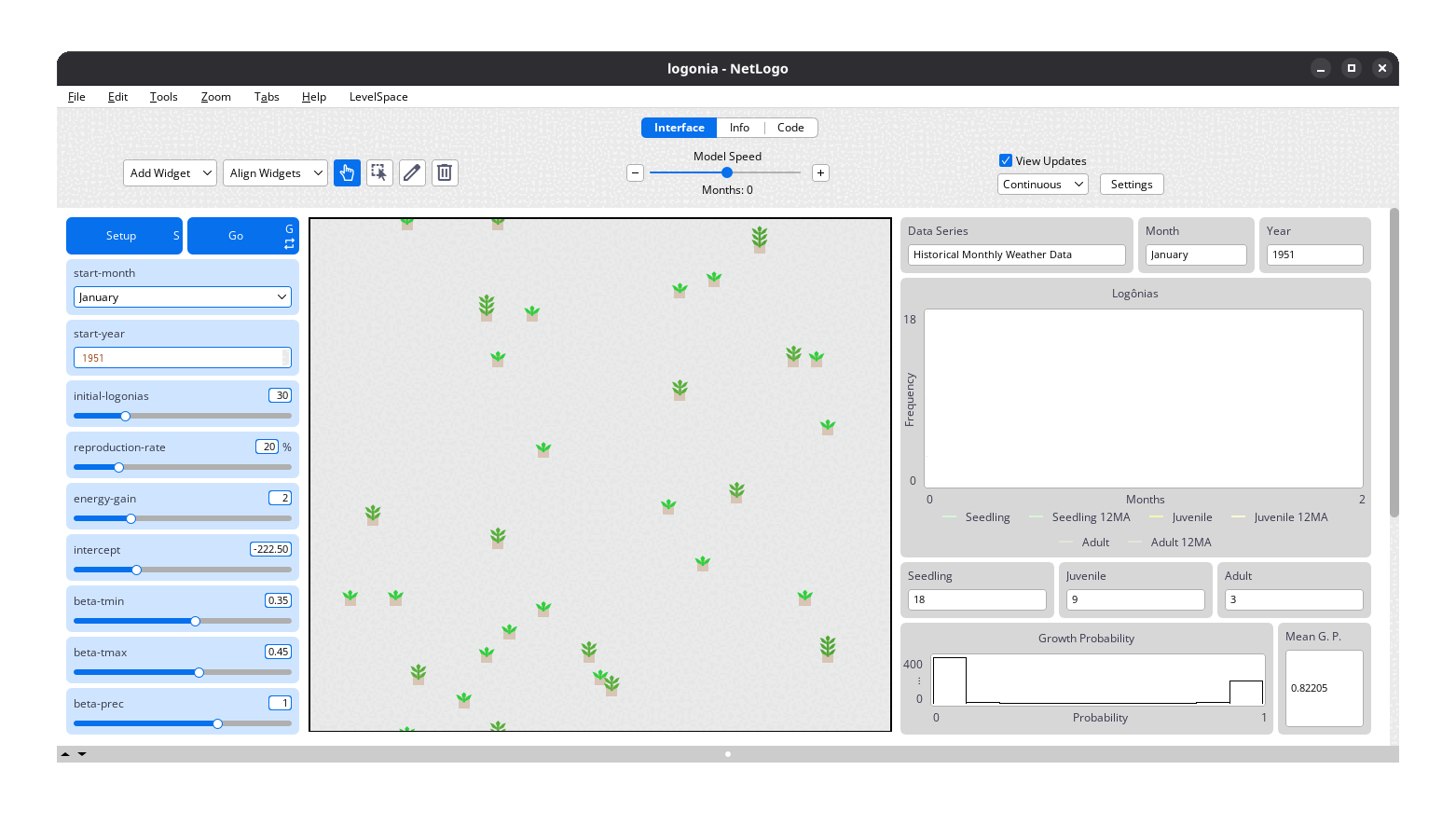
Logônia’s interface. Click on the image to enlarge it.